Polar equations often contain trigonometric functions. So you need
to understand the graphs of the basic trig functions and how to shift
and scale them. You can review by practicing with the following Maplets
(requires Maple on the computer where this is executed):
We have seen the graphs of a few simple polar equations. We want to be
able to graph more complicated polar equations. So we'll do it by examples.
The procedure is to make a table of points and/or make a rectangular plot
of the polar equation and use them to draw the polar plot.
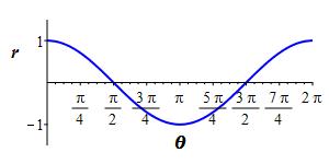
First think of \(r\) and \(\theta\) as rectangular coordinates.
The graph of \(r=\cos\theta\) is
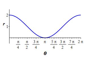
We lift this up by \(1\) so that the graph of \(r=1+\cos\theta\) is
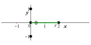
We first plot the polar points for these interesting points:
\(\theta=\)
\(0\)
\(\dfrac{\pi}{2}\)
\(\pi\)
\(\dfrac{3\pi}{2}\)
\(2\pi\)
\(r=\)
\(2\)
\(1\)
\(0\)
\(1\)
\(2\)
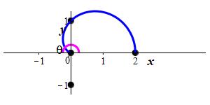
We now connect the dots in each quadrant. From the rectangular plot we
see that as \(\theta\) increases from \(0\) to \(\dfrac{\pi}{2}\),
the value of r decreases from \(2\) to \(1\). We add this to the plot:
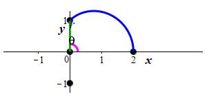
On the interval \(\dfrac{\pi}{2} \lt \theta \lt \pi\) we see that \(r\)
decreases from \(1\) to \(0\). We add this section next:
Finally, we see that as \(\theta\) increases from \(\pi\) to
\(\dfrac{3\pi}{2}\) to \(2\pi\), the value of \(r\) reverses and goes
from \(0\) to \(1\) and finally back to \(2\). We conclude
that the second half of the cardioid is a mirror image of the first.
This finishes the plot:
\(r=1+\cos\theta\)
Because it is shaped like a heart!
Watch an animation of the cardioid being drawn below.
\(r=1+\cos\theta\)
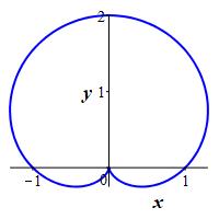
Plot the cardioid \(r=1+\sin\theta\).
\(r=1+\sin\theta\)
Frequently when plotting polar functions we allow \(r\) to be negative by
measuring backward. In particular, if the direction is \(\theta\), then
when \(r\) is positive, we move in the direction \(\theta\),
(and plot it in blue), but
when \(r\) is negative, we move in the direction \(\theta+\pi\),
(and plot it in red).
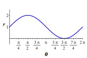
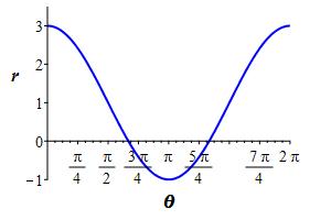
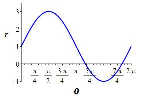
We follow the same procedure as last time by graphing \(r\) and \(\theta\) as
rectangular coordinates:
Notice that \(r=1+2\cos\theta=0\) when \(\cos\theta=-\,\dfrac{1}{2}\)
or \(\theta=\dfrac{2\pi}{3}\) and \(\dfrac{4\pi}{3}\). We add these to
the axes for our list of important points.
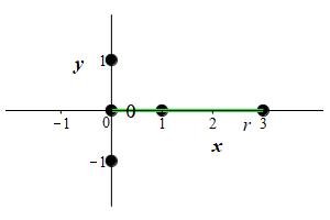
We plot the polar points at the important values of \(\theta\):
\(\theta=\)
\(0\)
\(\dfrac{\pi}{2}\)
\(\dfrac{2\pi}{3}\)
\(\pi\)
\(\dfrac{4\pi}{3}\)
\(\dfrac{3\pi}{2}\)
\(2\pi\)
\(r=\)
\(3\)
\(1\)
\(0\)
\(-1\)
\(0\)
\(1\)
\(3\)
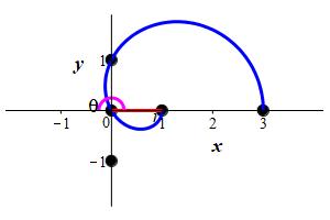
Notice that the origin occurs twice when \(\theta=\dfrac{2\pi}{3}\) and
\(\dfrac{4\pi}{3}\). Also when \(\theta=\pi\), which is the negative
\(x\)-axis, \(r=-1\) which we measure backwards along the positive
\(x\)-axis. Be careful to check that you know how each of these points
is plotted!
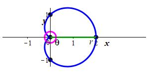
Next, we connect the dots by observing that \(r\) decreases from \(3\)
to \(0\) on the interval \(0 \lt \theta \lt \dfrac{2\pi}{3}\). Also
notice that \(r\) is negative on the interval
\(\dfrac{2\pi}{3} \lt \theta \lt \dfrac{4\pi}{3}\), so we measure \(r\)
opposite to the direction of \(\theta\) on this interval. The result
is plotted for \(0 \lt \theta \lt \pi\):
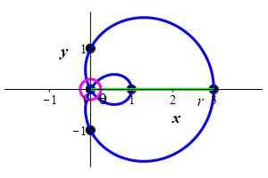
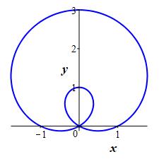
Finally, we note again that the second half is a mirror image of the
first. Thus by symmetry our final plot is:
\(r=1+2\cos\theta\)
The word limaçon is French for snail, but you can also remember that
it looks like a lima bean. View an animation of this limaçon being
plotted below.
\(r=1+\cos2\theta\)
Notice the radial line is
blue when the radius is positive and it is
red when the radius is negative.
Plot the limaçon \(r=1+2\sin\theta\)
\(r=1+2\sin\theta\)
When there is a multiple of \(\theta\) inside the sine or cosine, the horizontal
scale of the rectangular plot stretches or shrinks, changing the period.
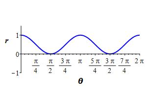
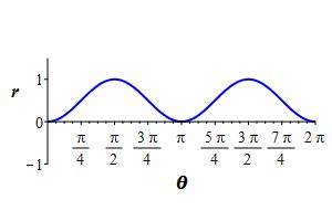
From the equation \(r=\cos^2\theta\), we find
\(r=0\) when \(\theta=\dfrac{\pi}{2}\) or \(\dfrac{3\pi}{2}\) and
\(r=1\) when \(\theta=0\) or \(\pi\). Also notice there are no negative
values of \(r\). The equation \(r=\dfrac{1+\cos2\theta}{2}\) makes it
easier to plot. Here is a table of important values and a rectangular plot:
\(\theta=\)
\(0\)
\(\dfrac{\pi}{4}\)
\(\dfrac{\pi}{2}\)
\(\dfrac{3\pi}{4}\)
\(\pi\)
\(\dfrac{5\pi}{4}\)
\(\dfrac{3\pi}{2}\)
\(\dfrac{7\pi}{4}\)
\(2 \pi\)
\(r=\)
\(1\)
\(0.5\)
\(0\)
\(0.5\)
\(1\)
\(0.5\)
\(0\)
\(0.5\)
\(1\)
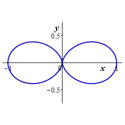
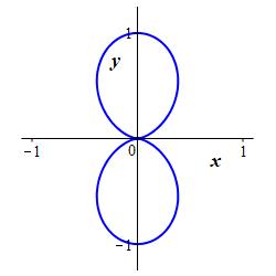
Notice the plot repeats with a period of \(\pi\). Here is the polar plot:
\(r=\cos^2\theta\)
Plot the curve \(r=\sin^2\theta\).
\(r=\sin^2\theta\)
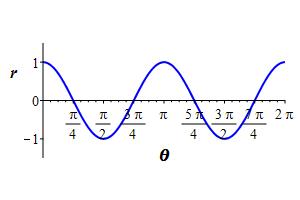
Now let's combine a change of period with negative values of \(r\).
Notice that \(r=0\) when \(2\theta=\dfrac{\pi}{2}, \dfrac{3\pi}{2},
\dfrac{5\pi}{2}\) or \(\dfrac{7\pi}{2}\) or
when \(\theta=\dfrac{\pi}{4}, \dfrac{3\pi}{4},
\dfrac{5\pi}{4}\) or \(\dfrac{7\pi}{4}\). Also \(r=1\) when \(\theta=0\)
or \(\pi\) and \(r=-1\) when \(\theta=\dfrac{\pi}{2}\) or \(\dfrac{3\pi}{2}\).
Also note that the plot repeats with a period of \(\pi\).
Here is a table of important values and a rectangular plot:
\(\theta=\)
\(0\)
\(\dfrac{\pi}{4}\)
\(\dfrac{\pi}{2}\)
\(\dfrac{3 \pi}{4}\)
\(\pi\)
\(\dfrac{5 \pi}{4}\)
\(\dfrac{3\pi}{2}\)
\(\dfrac{7 \pi}{4}\)
\(2 \pi\)
\(r=\)
\(1\)
\(0\)
\(-1\)
\(0\)
\(1\)
\(0\)
\(-1\)
\(0\)
\(1\)
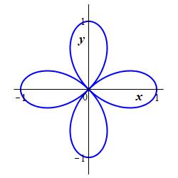
Also notice that the plot has \(2\) positive bumps and \(2\) negative
bumps in the interval \([0,2\pi]\). Here is the polar plot:
\(r=\cos(2\theta)\)
In the animation, the radial line is
blue when \(r\) is positive and
red when \(r\) is negative.
They trace out different leaves.
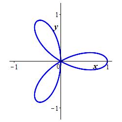
Plot the 3-leaf rose \(r=\cos{3\theta}\)
\(r=\cos(3\theta)\)
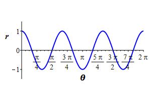
Here is a table of values and the rectangular plot:
\(\theta=\)
\(0\)
\(\dfrac{\pi }{6}\)
\(\dfrac{\pi }{3}\)
\(\dfrac{\pi }{2}\)
\(\dfrac{2\pi }{3}\)
\(\dfrac{5\pi }{6}\)
\(\pi\)
\(r=\)
\(1\)
\(0\)
\(-1\)
\(0\)
\(1\)
\(0\)
\(-1\)
There are \(3\) positive bumps and \(3\) negative
bumps in the interval \([0,2\pi]\). Here is the polar plot:
In the animation, the radial line is
blue when \(r\) is positive and
red when \(r\) is negative.
Notice that each leaf of the rose is traced
out twice, once when \(r\) is positive and once when \(r\) is negative.
How many leaves are there on the rose \(r=\cos(n\theta)\) if
\(n\) is even? Why?
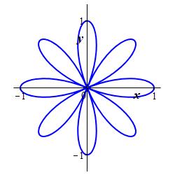
The rose \(r=\cos(n\theta)\) with even \(n\) has \(2n\) leaves.
For example, the rose \(r=\cos(4\theta)\) has \(8\) leaves:
\(r=\cos(4\theta)\)
Looking at the above example, we see that when \(n\) is even the polar plot
has \(2n\) leaves because \(r\) becomes negative at \(r=\dfrac{\pi}{2n}\)
and traces a leaf in the opposite quadrant before becoming positive again
at \(r=\dfrac{3\pi}{2n}\), and this repeats for \(n\) cycles. So \(r\)
traces \(2n\) leaves from \(\theta=0\) to \(\theta=2\pi\). For further
evidence, the polar plot of \(r=\cos(4\theta)\) is below, which has \(8\) leaves:
How many leaves are there on the rose \(r=\cos(n\theta)\) if
\(n\) is odd?
Why is this not the same answer as in the even case?
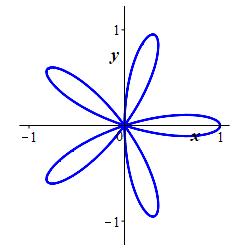
The rose \(r=\cos(n\theta)\) with odd \(n\) has \(n\) leaves.
For example, the rose \(r=\cos(5\theta)\) has \(5\) leaves:
\(r=\cos(5\theta)\)
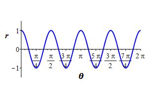
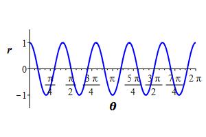
When \(n\) is odd the polar plot has \(n\) leaves because when \(r\)
becomes negative it overwrites a piece of the graph in the opposite
quadrant. For example, in the rectangular plot of \(r=\cos(5\theta)\)
below, there are \(5\) positive bumps and \(5\) negative bumps. Each
time \(r\) becomes negative, the graph retraces a leaf in the opposite
quadrant. So the polar plot has only \(5\) leaves.
You can review the graphs and equations of polar curves and practice identifying polar
curves from their graphs by using the following
Maplets (requires Maple on the computer where this is executed):
Placeholder text:
Lorem ipsum Lorem ipsum Lorem ipsum Lorem ipsum Lorem ipsum
Lorem ipsum Lorem ipsum Lorem ipsum Lorem ipsum Lorem ipsum
Lorem ipsum Lorem ipsum Lorem ipsum Lorem ipsum Lorem ipsum
Lorem ipsum Lorem ipsum Lorem ipsum Lorem ipsum Lorem ipsum
Lorem ipsum Lorem ipsum Lorem ipsum Lorem ipsum Lorem ipsum